It’s important to understand the math behind present value calculations because it helps you see what’s actually happening inside a calculator or spreadsheet. And once you understand the math, the calculations become much more intuitive. Yet, many people struggle with understanding present value formulas and calculations. In this post we’ll take a deep dive into the present value formula for a lump sum, the present value formula for an annuity, and finally the net present value formula for an irregular stream of cash flows.
Intuition Behind The Present Value
First, before getting into the actual math behind the present value calculation, let’s take a minute to think conceptually about the idea of the time value of money.
If I offer you the opportunity to have $1,000 today or $1,000 in one year, which would you choose? If you are a rational being, you will choose to take the $1,000 today. Why? Because there is risk associated with waiting to take the money in one year. I could lose all of my money, move away where you can’t find me, or die during the next year. In other words, there is a risk that you won’t actually get the $1,000 in one year.
The economic term for this concept is “risk aversion”, which means that all else equal, rational investors prefer less risk. In addition, if I give you the $1,000 today, you could also invest it for one year and have more than $1,000 at the end of the year. For these reasons, money has “time value”, which creates a mathematical relationship between present value dollars and future values dollars. Let’s take a closer look at this relationship in order to derive the present value formula for a lump sum.
Present Value Formula For a Lump Sum With One Compounding Period
This brings us to the topic of interest and interest rates. As a rational, risk averse investor, you require some additional compensation in order to wait a year to receive your money. The amount of additional money you require to wait is an implicit measure of your personal interest rate. That interest rate represents a measure of lost investment opportunity cost, market risk, and investment-specific risk. Let’s assume that you agree to wait one year to receive your cash if you are promised $1,100, or an interest rate of 10%. Mathematically, this calculation shows that the future value (FV) is equal to the present value (PV) plus the additional interest you require as compensation for time and risk (PV * R).
$1,100 = $1,000 + ($1,000 * .10)
FV = PV + (PV * R) = PV (1 + R)
This time value of money concept and mathematical relationship is central to understanding the present value calculation. It also lets us consider the opposite relationship, or how present value relates to future value. For example, how much would you be willing to pay today for the promise of $1,100 in one year? Using the same required rate of return, 10%, we can calculate that the value of that investment today is $1,000.
PV = FV / (1+R)
$1,000 = $1,100 / 1.10
Present Value Formula For a Lump Sum With Multiple Compounding Periods
In the previous example, the interest rate only had one compounding period. Most investments, however, compound interest more frequently than once each year. Monthly or daily compounding of interest is far more common than annual interest compounding. Investors also benefit from the increased frequency of compound interest.
Consider how the calculation of future value in our example above would change with semi-annual compounding. Instead of one compounding period, there are now 2 per year. So, the stated 10% interest rate is divided by the number of compounding periods, and the number of compounding periods likewise increases. That means we earn 5% per period for a total of 2 periods now.
In the first period the $1,000 increases by 5% to $1,050, and in the second period the $1,050 earns another 5% interest for a total of $1,102.50.
Period 1:
$1000 (1.05) = $1,050
Period 2:
$1,050(1.05) = $1,102.50
In other words, the formula adds another component (N) to represent the number of compounding periods.
1,102.50 = $1,000 (1 + 10/2)2
FV = PV (1 +R/N)N
PV = FV / (1 + R/N)N
As an aside, notice how increasing the frequency of compounding also increases the actual realized rate of return. In this example the stated interest rate was 10%, but the realized annual rate of return was $102.50/$1,000, or 10.25%. This actual, realized rate of return is known as the Effective Annual Rate (EAR).
Present Value Formula for an Annuity
You can then extend this basic mathematical framework to calculate the present value of more than one cash flow. Consider the basic model where interest was compounded annually and you would receive a payment of $1,100 in one year. Now you will also receive a payment of $1,100 at the end of the second year. The present value is now the sum of discounting one payment of $1,100 back one year to the present as well as one payment of $1,100 two years back to the present.
PV = 1,100/(1.10)1 + 1,100/(1.10)2 = $1909.09
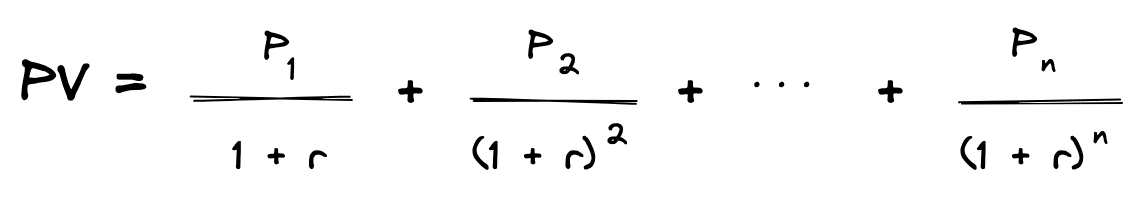
If all of the payments stay the same, meaning here you are getting the same $1,100 every period, there is a special way to combine all of those terms into a formula known as the present value of an annuity. The numerator of the fraction (the $1,100) does not change, and the only part of the formula that does change is the number of periods a particular cash flow gets discounted (the exponent on the 1.10 in the denominator). The generalized formula for present value of a stream of cash flows is represented in the following equation where P is the payment or cash flow received during the period, R is the periodic rate of return, and N is the number of periods.
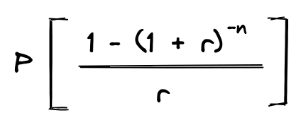
Mathematically, this is also known as a geometric series. When each of the cash flows is the same (P), there is a special way that the discount factors can be simplified. In this case, the present value equation can be simplified like this:
Net Present Value Formula For an Uneven Stream of Cash Flows
While the above present value of an annuity formula is helpful for valuing an annuity or a mortgage loan in which the payment does not change, this formula is not particularly helpful when computing the value of an investment with varying cash flows. The mathematical concept of discounting future cash flows back to the present time does not change, but we give the formula a different name. The net present value formula simply sums the future cash flows (CF) after discounting them back to the present time.
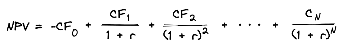
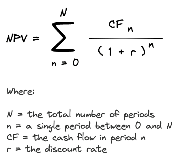
The formula for net present value also accounts separately for any initial costs incurred at the beginning of the investment (CF0). Since the amount of the cash flows changes, this formula cannot be reduced to a simple geometric series. So, the net present value formula can be simplified as follows:
Example
Net present value calculations are an essential tool when calculating the value of commercial real estate. For example, suppose you have the proforma cash flow statements for a property and want to estimate a reasonable purchase price today. Net operating income is estimating to be $35,000 in year 1, $37,000 in year 2, $38,000 in year 3, $40,000 in year 4, and $41,000 in year 5. After holding the property for five years, you expect the sales price to be $450,000. You have a required rate of return equal to 8%. So, you use the following equation:
NPV =35,000/(1.08)1 + 37,000/(1.08)2 + 38,000/(1.08)3 + 40,000/(1.08)4 + 491,000/(1.08)5
NPV = $457,862
In other words, your estimated value of this property is $457,862. The value today is determined by the estimated cash flows you expect to receive in the future after being discounted back to the present time using an interest rate that represents your uncertainty (risk aversion) about the amount and timing of those cash flows.